Twice Told Tale: Properties and Applications of the 2D Fourier Transform

Anamorphic Property of FT of 2D patterns

Anamorphic property of FT is shown where a wide pattern has a long FT and a long pattern has a wide FT. This is shown in figure 1. Also, two dots along x produces a sine along y.

Figure 1. Anamorphic property of FT. The left panels refers to the 2D patterns. The right panels refers to the FT of each pattern. a) Tall rectangle apperture produces a wide FT. b) a wide rectangle aperture produces a tall FT. c)  Two dots along x-axis symmetric about the center produces an airy pattern with a superimposed sinusoidal signal along y.  d) The frequency of the sinusoidal signal decreases when the spacing between the dots is decreased.

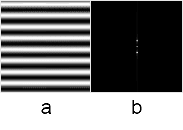
Rotation Property of the FT

For a sinusoidal signal, the produced FT will be two peaks centered at zero. The peak corresponds to the frequency of the signal. Higher frequency shows that the peaks move farther away from the center as shown in figures 3 and 4. A constant signal will have an FT with a peak at zero since a constant signal can be thought of as a sine with a very low frequency. Therefore, when a sine has a constant bias, a peak at the center will be observed in the FT. When the bias in a sine is also a sine with a lower frequency, peaks nearer the center will be observed in the FT, corresponding to the frequency or the bias. These are all seen in figure 2. In this case, the higher peaks corresponds to the frequency of the main sine signal. So for sinusoidal signals with bias, to obtain the frequency of the main sine signal, a low pass filter can be used mask off the peaks near the center and to isolate the peak corresponding to the main signal.

Figure 2. FT of sines. Left panels refer to the sinusoidal signals. Right panels refer to the FT. a) Sine centered at zero. The FT has two peaks along y centered at zero. b) Sine with a contant bias. FT aside from the two symmetric peaks, also has a peak at zero. c) Sine with a sinusoidal bias. FT has a peak at zero, two small peaks near the origin, and another two far from the origin.

Figure 3. FT of a sinusoid while increasing frequency. Increase in the frequency of the sine shifts the peaks in the FT farther from the origin.

Figure 4. FT of the sinusoid wil a constant bias. A peak at the center can be observed.

A rotated pattern produces an FT rotated in the same direction. This can be observed in figure 5. 

Multiplication of patterns produces an FT which is a convolution of the FT of the individual patterns. Figure 6(a) shows the multiplication of a sinusoidal along x and a sinusoidal along y. The FT of a sinusoid along x are two deltas along y, and the FT of a sinusoid along y are two dirac deltas along x. The produces FT in figure 6(a) left panel is a convolution of two dirac deltas along x with two dirac deltas along y. Combining this again with a rotated sinusoid produces an FT with peaks along a rotated axis. 

Figure 5. Rotating the sinusoid rotates the FT at the same angle. 

Figure 6. Combination of sinusoids. a) Combining a horizontal and a vertical sinusoid (right panel) produces a FT with peaks along X and along Y. b) Combining a rotated sinuoid with the figure in (a) (right panel) produces the same FT but now with peaks along a rotated axis. 

Convolution Theorem Redux

In this part the convolution will be more emphasized. The FT of two dirac delta of one pixel as a peak, is a sinusoid. Convolving a dot of some radius with the dirac delta has an Airy pattern with a superimposed sinusoidal FT. For a square convolved with the two dirac deltas, the FT is a sine along x and along y with a superimposed sine signal. For a gaussian convolved with the two dirac deltas, the FT is a gaussian superimposed with a sine signal. This are all shown in figure 7. Increasing the size of the shape convolved with the two dirac deltas, decreases the size of the FT, as can be seen in figures 8-10. 

Figure 7.  The 2D patterns (left panel) and its FT (left panels). a) binary image of two dots with one pixel each produces a very big FT with a superimposed sine. b) Replacing the dots with circles produces an Airy pattern with a sine of the same frequency. c) Replacing the dots with squares produces a sinusoidal along the center of x and y with a super imposed sine of the same frequency as in (a) and (b). d) replacing the dots with gaussians produces one gaussian with superimposed sine same as in (a), (b), and (c). 

Figure 8. FT of two dots with increasing radius. The size of the FT is inversely proportional with the radius of the circle. 

Figure 9. FT of two squares with varying width. The thickness of the FT is inversely proportional to the width of the squares. 

Figure 10. FT of two gaussian is a gaussian with a super imposed sine. Increase n the variance of the gaussian decreases the size of the FT. 

Figure 11 shows the effect of the convolution of a pattern with a dirac delta. This results to an imprint of the pattern at the location of the dirac delta. Figure 11 a) is the convolution of randomly placed dirac deltas with a paw print and a mickey mouse head. Note that the resulting convolution has an increased dimension with the original. The convolution of an NxN matrix with dirac deltas with an nxn pattern results to an N+n-1 by N + n-1 matrix. The placement of the pattern is the relative location of the dirac delta with the center. The convolution in figure 11 a) can be used as an acitivity for finding the hidden mickey. Figure 11 b) is a more challenging convolution since the r, g, and b channels has to be preserved. To do this, I convolved the R, G, and B channels of the colored flower pattern with the randomly placed dirac deltas shown in the left panel. The background of each colored flower pattern was segmented using a threshold. The segmentation however is not perfect especially for the white flower since the background of each colored flower pattern is white. A mask was made so that areas already placed with a flower will not be added with another pattern. Without the mask, the colors of the flowers will be destroyed, since the steps were done separately for each R, G, and B channel. Figure 11 c) increased the dirac deltas and the flower patterns. This method could be used for fast creation of colorful floral patterns. 

Figure 11. Convolution of a pattern (right panels) with dirac deltas at random locations (left panels). 

Equally spaced dirac deltas produced equally spaced FT. The spacing however is opposite for each FT pair. A widely spaced pattern will have a narrowly spaced FT. This is shown in figure 12. 

Figure 12. FT of equally spaced ones. The increase in the spacing of the ones in the pattern produces a decrease in the spacing of the ones in the FT. 

Fingerprints: Ridge Enhancement

For a fingerprint, the information are in the ridges of the pattern. The fingerprint however has ink blotches, making the pattern inaccurate. To recover the ridges in the fingerprint, a mask can be used in the FT to preserve the circular peaks corresponding to the ridges. This is shown in figure 13. 

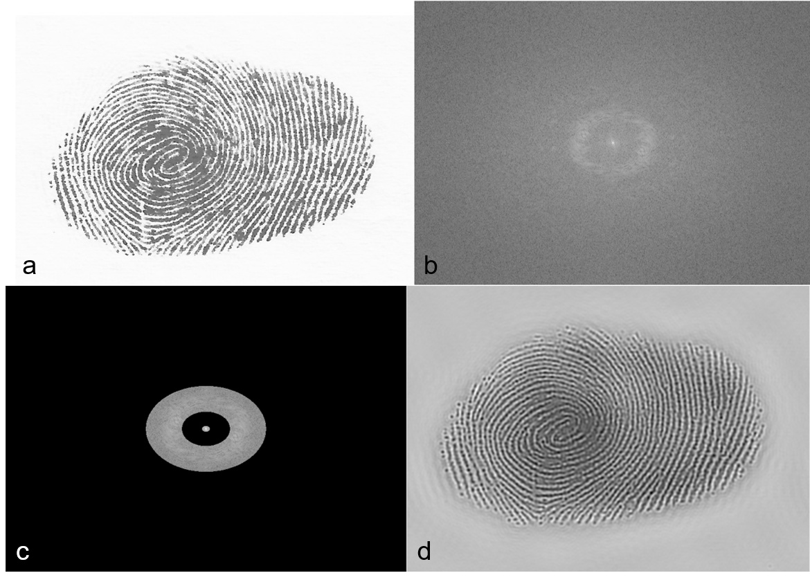
Figure 13. Ridge enhancement of a fingerprint. a) The fingerprint. b) The FT showing a circular ring near the center. c) Isolating the circular ring and the peak at the center using a mask. d) The inverse FT of (c) capturing the ridges of the fingerprint. 

Lunar Landing Scanned Pictures: Line removal

Repeating lines can also be removed with the knowledge that the FT of repeating lines are peaks along x or along y. A mask covering the peaks spanning vertically and horizontally in the FT can be used as shown in figure 14. The resulting image from the inverse FT in figure 14 d) shows a cleaned image where the lines were removed. Care should be observed however since some sharp edges which are part of the picture got smoothed out due to some removed signals in the image. 

Figure 14. Line removal of a lunar landing image. a) The scanned image. b) The FT showing peaks spanning horizontally and vertically along the center. c) Removing the peaks using a mask. d) The cleaned image. 

Canvas Weave Modeling and Removal

For paintings or other materials printed in a canvas, the texture of the canvas messes up with the information contained in the material. From scanned painting, there is a repeating pattern which seems to be not included in the painting. This repeating pattern is similar to the patterns in figure 6. A mask should be created to remove twin peaks of the combined sinusoidal signals. Figure 15 d) shows a clean image. The FT of the peaks removed by the mask, is a weave pattern as shown in figure 15 e). 

Figure 15. Removal of canvas weave in a scanned painting. a) The painting. b) the FT of the image. c) Removal of the peaks corresponding to the canvas using a mask. d) The cleaned image. e) The inverse FT of the peaks removed in (b). f) The result of subtracting the cleaned image from the original image. 

For this work, I give myself 10/10 since i completed all the necessary activities. I would like also acknowledge Justin, Chloe and Ado for helping me with some parts.

Mark Twain once said that history doesn't repeat itself, but it does rhyme. - Albert-László Barabási

Through Rose-Colored Lenses: Color Image Segmentation

For this activity, objects in an image can be detected using its color. This is very easy for humans, now, we will let the computer do it using normalized chromaticity coordinates. The first method is to do parametric segmentation where the value in a gaussian distribution of each pixel was obtained using the mean and the standard deviation of the region of interest. Basically, this shows how is the color of the pixel from the color of the ROI in the NCC plot.  

Non-parametric segmentation uses the NCC plot of the region of interest. For each pixel in the original image, the (r,g) values will be obtained. The frequency of the (r,g) value in the NCC plot of the ROI will the new pixel in the converted image. The converted image will then have white or high pixel values for objects with colors same as in the ROI.

Figure 1. The original image used. 

Figures 2-6 shows different results of segmenting the image using different ROIs. One common observation is that the non-parametric segmentation captures other objects with colors included in the region of interest. The parametric segmentation only objects with colors very near to the color of the region of interest. In figure 2, for example, the parametric segmentation captured brightly the blue logbook only. It faintly detected the blue shirt at the lower left of the image. The non-parametric segmentation also captured the cyan rose notebook and the cyan pen near the center. 

In figure 3, the cyan pen was also detected by the non-parametric segmentation. 

In figure 4, the parametric segmentation detected the red notebook and the pink container at the left. The floor, the umbrella, the roses, and other reddish colors were not detected but were detected using the non-parametric segmentation. 

In figure 5, only the yellow notepad was detected, other instances of yellow were not detected by the parametric segmentation, but were detected by the non-parametric segmentation. 

Figure 6 is a bit hard since the region of interest contains more than 1 color. Focusing on the region of interest, which is the rose notebook, parametric segmentation faintly detected the notebook. Black and white images however were brightly captured even though the ROI is not abundant in black and white pixels. Non-parametric segmentation brightly captured the region of interest and also captures other objects with cyan or red tint. 

For object tracking, parametric segmentation might be more ideal since it only focused on the most abundant color in the object. There is lesser noise in the background. For color tracking however, non-parametric segmentation is better since it detects instances of the colors in the ROI. Parametric segmentation works best when the ROI is monochromatic. For an ROI with more than one color, parametric segmentation detects white or black pixels since it is near the center of the NCC. In this cases, it is better to use the non-parametric method. 

Figure 2. Segmenting the blue logbook. a) The ROI and the NCC histogram. b) Parametric segmentation. c) Using the result of the parametric segmentation as a mask isolates the notebook. d) The NCC histogram of the original image. e) Non-parametric segmentation. d) Non-parametric segmentation as a mask. 

Figure 3. Segmenting the green logbook. a) ROI. b-c) Parametric segmentation. d) NCC histogram of the original image. e-f) Non-parametric segmentation. 

Figure 4. Segmenting the red notebook. a) ROI. b-c) Parametric Segmentation. d) NCC histogram of the original image. e-f) Non-parametric segmentation. 

Figure 5. Segmenting the yellow notepad. a) ROI. b-c) Parametric segmentation. d) NCC histogram of the original image. e-f) Non-parametric segmentation

Figure 6. Segmenting the Rose notebook. a) ROI. b-c) Parametric segmentation. d) NCC histogram of the original image. e-f) Non-parametric segmentation. 

For this activity, I give myself 10/10 since I completed the whole activity. I would also like to acknowledge Rey and CJ for the image used, which is the image we used for a group activity in 187.

No matter what anyone says or does, my task is to be emerald, my color undiminished - Marcus Aurelius

I open at the close: Morphological Operations

Morphological operations is one of the subjects I really like in 186. I think it should be taught earlier next to image segmentation. During my BS3 days, I struggled on processing a video of a pile of grains with only google skills and no image processing knowledge. At first, I was to track the spaces between the grains. This is quite easy for me since I can use region props. However, when tracking the actual grains, all the grains is in one huge connected component, where region props is pretty useless. It eventually reached the limitation of my google skills and I made no progress on it since then. But lo and behold, morphological operations!!

From the word morphology, referring to shape or structure, a structuring element expands of reduces a shape using dilation and erosion. Combination of dilation and erosion creates new useful morphological operations, which are the closing and the opening operator. The closing operator dilates then erodes and the opening erodes, then dilates. The available tophat function obtains the blobs removed by the opening operator. The closing operator in general ‘closes’ an object or removes the holes inside a shape. The opening is used for cleaning the scattered noise in an image. With this in mind, one can think of using morphological operators to ‘clean’ an image after binarization. I could now go back to A6 to clean the edge detection technique I did. 

There are two main morphological operation, which is the dilation and erosion. Other morphological operations are combinations of these basic operation. Dilation of a shape with a structuring element consists of the intersection of the shape and the translation of the structuring element with the shape. Translation here referes to the area covered when the point of reference of the structuring element traverses the whole shape. Dilation makes the shape expand. Erosion in the other hand can be thought of as the area reached by the point of reference in the structuring element while the structuring element moves inside the shape. This operation reduces the shape. 

For the following shapes: a 5x5 square, a triangle with a base of 4 and a height of 3, a hollow 10x10 square of 2 boxes thick, and a plus sign of 1 thickness and 5 pixels along each line, a dilation and erosion of the following structuring elements: 2x2 ones, 2x1 ones, 1x2 ones, and a cross of 3 pixels long and one pixel thick was done by hand and was plotted using Matlab. The results are shown in figures 1, 2, 3, and 4. The rendered images in matlab was inverted to show the shaped form using black pixels instead of white. Most of the resulting shape manually made are similar to those rendered. For the dilation of the triangle with the cross however, there is a slight difference. This could be due to the limitation of the rendering, where the program tends to smoothen the images when there is an edge. 

Figure 1. The dilation and erosion of the shapes 5x5 square, a 4x3 triangle, a 10x10 hollow square and a 5x5 plus sign with a 2x2 structuring element. 

Figure 2. The dilation and erosion of the shapes with a 2x1 structuring element 

Figure 3. The dilation and erosion of the shapes with a 1x2 structuring element

Figure 4. The dilation and erosion of the shapes with a 3x3 cross structuring element

For the application, we now use the morphological operations in an image of circles. In this, we pretend that the circles are normal sized cells. The area of the normal sized cells should be known in order to locate the abnormally sized cells which could possibly be a cancer cell. So, we binarize the image first using a threshold from the histogram of the image. The peak at the histogram shows the pixels of the background, which is the most abundant pixels. I chose the upper limit of the curve as the threshold to perfectly eliminate the background. In this part, I would like to acknowledge Sir Mario since he saw the bug in my code regarding histogram, in which I was stuck with for days.

Figure 5. The section 7 of the image a) the section 7 b) the binarized image based on the threshold obtained from the PDF c) The PDF of the intensity values of the image. The threshold used was 205, which is at the upper limit determining the pixels of the background.

Figure 6 refers to the sections in the segmented image. Some sections have overlapping areas. For the binarization, shown in figure 7, a different threshold was used for each subsection depending on the histogram of the image. The threshold obtained are just estimated and the range is small, which is from 200 to 218. Using a constant threshold value for all would seem okay. With this method however, some blobs get distorted and gets eliminated after morphological operations. Some blobs also gets merged and turned into a very big blob which is lost data since we need statistics of the area of the cells. To solve this, two methods could be done: 1) personalize the morphological operation used for each section or 2) personalize the threshold values. The result of personalizing the threshold value for each subsection is better since after the morphological operation, fewer blobs got merged. The best result was shown in figure 7, and will be used to the next processes.

After binarization with the best threshold values for each subsection, the images are still not it its ideal look. In figure 7, there are still observable residue from the binarization made. This is more visible in the small white noise-like dots in the middle subsection (section 5) and the lower left subsection (section 7). This is now where the morphological operations are used, which is already repeatedly mentioned since the start. The best result is shown in figure 8, where opening was done first to remove the small dots, then closing, to remove holes in the blobs. The structuring element used is a disk with a radius of 2-5 pixels for both operation.  The structuring element was made to be smallest as possible since at a bigger radius, the blobs became deformed and most of the blobs gets merged, which is lost data. Care should be taken however since at a very small radius, the small white dots does not get removed after opening. Also opening first rather than closing gives out a cleaner result since if closing was done first, the small white dots expands with a big structuring element. When closing with a small structuring element, the holes inside some of the blobs does not get removed. Another problem is that some of the noise in the background grows bigger as seen in the upper left image (section 1).

Figure 6. The image divided into 9 256x256 sections

Figure 7. The image binarized in each subsection. The threshold use for each subsection varies depending on the obtained histogram of the image. For left to right, top to bottom subsections, the thresholds are 210, 213, 220, 200, 200, 218, 205, 205, 220. 

Figure 8. The image applied with morphological operations. First, it was applied with opening, to remove the small dots, then  closing, to remove a few holes inside the blobs. 

It is a sad thing not to be able to separate the the merged blobs. There is another morphological application that can do this. It is the watershed segmentation, which was mentioned in my previous post. I will try to do this, if there are still time. For now, the available data from the isolated cells would suffice.

Each blob was labelled and separated using connected components. The area and radius of each blob was obtained using properties from regionprops. From the labelling done, one blob can be individually displayed as shown in figure 9. The histogram of the areas of the blobs is shown in figure 10, here, the abnormally sized cells were already removed. The threshold value for removal was estimated from the histogram of the original data. 

Figure 9. The blobs in section 7. a) The connected components was separated by looking at the connected white pixels bounded by black pixels as one component. b) each connected component was labelled as shown by the different colors when endered with imshow. c) One blob can be separately shown using the label. 

Figure 10. The PDF of the areas of the cells. The abnormal sizes were already removed. The mean area of the blob is 505.900 px and the standard deviation is 2.9230 px. The mean radius estimate of the included blobs was computed to 14.9869 px with a standard deviation of 2.9230px.

Now, to remove isolate the cancer cells in an image, the opening operator was applied to the image using a structuring element of a disk with a radius of the mean radius of the normal cells. With this operation, the structuring element buries the shapes of the same size during erosion, removing it completely. A bigger structuring element will remove the cancer cells while a smaller one will not completely remove the normal sized cells. Figure 11 shows this step. In figure 11 e) only the cancer cells remained. Using manual checking, 5 abnormally sized cells can be detected in the original image. This shows that the method is good. 

Figure 11. The image with cancer cells. a) The binarized image. b) Image after opening. c) image after closing. d) The different labels of the blobs. e) opening with a disk of radius 15, which is the mean radius of normal cells.

For the activity, I give myself 10/10 since I have completely done all the expected output and the images looks good. Aside from all the many people who helped me finish this activity, I would specifically thank Kuya Franco for mentioning the function strel in matlab. Without it, I was manually creating matrices for my structuring element.

The worst prison would be a closed heart – John Paul II 

Moment Frozen in Time: Basic Video Processing

The last 186 activity for me is the one big aspect of image processing. It comes from the idea that a video is a series of images. Individual image processing of each frame in a video is video processing. In this activity, we were tasked to do a common physics experiment done in video and do the analysis using image processing of the video frames.

For each video, it is vital to know the frame rate of the video, or the number of frames flashed per second, especially when temporal information is needed. The ideal frame rate to prevent lost of information is based on the Nyquist Criterion. 

For this activity, we did a classic physics free fall experiment, which we all know by heart. A video captured a free falling tennis ball for 29.97 frames per second. The frame rate is okay since there is no repetitive motion. 

In the experiment, the acceleration due to gravity can be measured by obtaining the change in speed of the tennis ball over time. To do this, the location at every instant of the tennis ball should be obtained. 

From the video, image segmentation was used to locate the tennis ball using the ROI from the surface of the tennis ball at one frame. Since this is a video, the quality of each frame depends on the frame rate. Most of the frames made the ball look blurry especially towards the end where the speed is increasing. Seen in figure 1, at frame 50, the ball is so blurry and is almost unseen. With this, care should be taken when choosing the ROI. When an ROI is from a frame where the object is not yet moving, the ball gets undetected at a later time since the ball blurs. In my case, the ROI is from frame 47 since the color captures the motion of the ball but is not so blurry that the background would be selected. Further improvement in the tracking is done using morphological operations. Regionprops was used to detect the centroid of the ball, which tells the approximate location at that frame. 

Figure 1. Frames 47 and 50 of one trial of the free fall video. 

The videos below show one of the trials done. The center of the white blobs show the pixel locations of the ball, which was converted to actual coordinates from the pixel length of the protractor which is 12.5cm. The corresponding frame at which the ball was located was also converted to real world time coordinates from the frame rate property of the video. 

The tracked positions of the tennis ball for 4 trials are shown in figure 2. The speed is shown in figure 3. The position was adjusted so that the floor is at 0m. This adjustment is needed since the pixel convention is increasing from top to bottom. From the curve fit of the trajectory, the acceleration due to gravity has the values of -8.37 m/s², -9.22 m/s², -10.11 m/s², and -9.45 m/s². The obtained values are near the accepted value. Deviations from the measurement could be due to the blurring of the ball while in motion. From the velocity plot however, shown in figure 3, the acceleration values are 9.79m/s², 9.73 m/s², 7.18 m/s², and 7.96 m/s². For each trial, the obtained value if different for the two plots. The lines in figure 3 however do not fit well as shown by the r² values from 0.6 to 0.7. For trial 2, shown by the orange plots in figures 2 and 3, the obtained values for the acceleration are close to each other, which is 9.22 m/s² and 9.73 m/s². Interestingly, the r² of the fit in the velocity plot is 0.93, which is close to 1. Interestingly, the obtained values for the acceleration. The disparities of the computed values could be due to the blurred motion of the ball caused by the limitation of the camera and the video's frame rate. 

Figure 2. The position vs time plot of the tennis ball in free fall. Curve fitting gives the value of acceleration of -10.11 m/s² to -8.37 m/s²

Figure 3. The velocity vs time plot of the tennis ball in free fall. Linear regression obtains the acceleration values in the range of 7.18 m/s² to 9.79 m/s².

I really like this activity since in some of our Physics 19x experiment, we were forced to do image processing for the data analysis due to the limited working lab quest available. I had fun in video analysis and object tracking since some of the data, such as the swinging of the pendulum, or the collision of two objects, etc, are hard to see using the naked eye, but is very observable when the videos are sliced into frames. 

For future work, it would have been more fun to do some pendulum experiment such as the energy transfer experiment in 191. This experiment requires focus from the experimenters since the amplitude of the pendulum swing varies and some set-up has very fast energy transfer. It is also hard to use a motion detector for this since there are two pendula and their sync is essential. Also, with pendulum experiments, only the frame rate is important for conversion to real world coordinates. The pixel to real world distance is most of the time not needed. 

For this activity I failed to do an additional exploration part due to the limits of time. However, in my future works, I will still do more object tracking and video analysis. It also took me a little longer than expected to finish this activity since the ruler, seen in figure 1, gets segmented with the tennis ball, and it took me a while to solve the blurring of the ball, which made it undetected. Despite that, I think I perfectly understand the concepts needed for this activity, and the plot and videos are good. I also had a few practice with using videoWriter() function and in obtaining a good frame rate but I turned the video into a gif file since blogger lowers the quality of the video. So I give myself 10/10 for the evaluation. 

I would like to thank Nica and ate Clei for letting me help in the acquisition and sharing with me the experiment video. I also acknowledge all the other people who helped me learn things in this 186 course, which I used in finishing this activity. 

It does not matter how slowly you go as long as you do not stop. -Confucius

Fourier for Today: Fourier Transform Model of Image Formation

Fourier transform is a wonderful linear transform which converts a signal into its inverse dimension. For a signal with dimensions of space, FT converts it to a signal of spatial frequency. For a 2D image, the FT is given in the equation below.  A powerful implementation of FT is the fast fourier transform algorithm which is fft2() in matlab and something similar in other packages. This function however has different properties and we should be careful in using them.

For our 186 subject, it is a required skill to be familiar with and to know by heart the fourier transform of different patterns. There are a few get away tips to easily familiarize oneself on FT. first is that the FT of a pattern is in inverse dimension of those of the pattern. From here, we can say that when the pattern is long then the FT is short or when the pattern is short the FT will be long. The FT of a small aperture will be wide. Second is that when the pattern is rotated, the FT will be in the same rotation. Last is that the product of two patterns will have a FT of the sum of the individual FT of the patterns. It is also important to note that the FT of an FT of a pattern is the pattern itself, so a pattern and its FT is somehow like a pair. So now, we look at FT of some basic patterns. 

Figure 1 shows the FT of a circle. 1(a) is the circle. This pattern could be thought of as a circular aperture. Figure 1(b) is the output of the FFT algorithm, which is not yet center shifted. This should always be noted in using FFT algorithms from packages. The function fftshift() can fix it. Figure 1(c) is the FFT of the circular aperture, which is an Airy pattern. Note that the pattern is medium sized, producing a medium size FT. Figure 1 (d) is the FT of the Airy pattern in figure 1 (c) showing that the FT of the FT of the circle is a circle. It should be noted also that the FT of a function is complex. Figure 2 shows the real and imaginary parts of the FT. 

Figure 1. The FT of a circular aperture. (a) the circular aperture. (b) The pattern produced by the FFT algorithm. (c) The FT of the pattern. (d) the inverse fourier transform of the FT. 

Figure 2. The complex FT of letter A. (a) the pattern A. (b) The FT of the pattern. (c) The FT of the FT of the pattern. (d) The real part of the FT of the pattern. (e) The complex part of the FT of the pattern. 

Figure 3. a) A sinusoid along x (corrugated roof) b) The FFT of the sinusoid which is a two dirac deltas and a direct delta at the center 0. 

Figure 3 shows the FFT of a sinusoid along x, which is a two dirac delta with peaks corresponding to the frequency of the sinusoidal signal. For the fourier series, any signal can be expressed as a linear superposition of weighted sines and cosines of different frequencies. The fourier transform shows the distribution and the relative strengths of sinusoids in the signal. In this case, the frequency as which the sinusoid was made is at the peak of the dirac delta, which is the sinusoid with the highest strength. The spread of the dirac delta shows the other available signals. A constant signal is like a sinusoid with a very low frequency, which has an FFT of dirac deltas very near the center 0. So for a constant signal, the FFT is at the center. A double slit however, as seen in figure 4, can be thought of as a many dirac delta signals along the y axis centered at x = 0. It’s FFT will be a sinusoid along x-axis. Another signal that can be thought of as a superposition of many sinusoids is a square pattern. The FFT is a sinusoidal signal forming a cross. Since the square is wide along x and along y, the FFT is thin and long along x and y. 

Figure 4. The double slit and its FFT which is a sinusoid along the x-axis but confined only along y = 0.

Figure 5. Square and its FFT, which are sinusoids along x and y forming a cross

A Gaussian bell curve will always have a Gaussian as its FFT. A small pattern will have a big FFT. This is shown in figure 6. 

Figure 6. The FFT pair which is a small and big 2D Gaussian bell curve

Simulation of an imaging device

Convolution is used in imaging such that the resulting convolution of 2 patterns looks like both the 2 patterns. The result is like the smearing of one pattern to the other. For an object, the resulting image taken by an imaging device is the convolution of the object and the transfer function of the imaging device.

It is also essential to note that the FFT of a convolution is the product of the individual FFT of two patterns. With this in mind, to determine the FFT of a difficult pattern, the pattern could be broken down to easy patterns with known FFT and obtain the product of the FFTs.

In the next part, we will simulate an imaging device. For a digital camera for example, the finite lens radius limits the gathered rays reflected from the object, making the reconstruction imperfect.

We have an object which is the letters VIP in Arial font. The imaging device is shown by a white centered circle. In figure 7, radius of the imaging device was increased from left to right. The increase in the radius of the imaging device reblurred the reconstructed image. The greater the radius, the better the quality of the produced image. This can be observed also in a video bellow where the radius of the aperture increases. 

Figure 7. The convolution of the letters VIP and a circle with varying radius. a) r = 0.1 b) r = 0.3 c) r = 0.5 d) r = 0.7 e) r = 0.9

Template matching using correlation

Correlation is another tool used to look into the degree of similarity of two patterns. The high the correlation at a certain pixel implies that the patterns are identical at that point. This can used for template matching or pattern recognition. For the activity, we used a template with the text: “THE RAIN IN SPAIN STAYS MAINLY IN THE PLAIN” in Arial 12. The letter “A” typed also in Arial 12 was correlated with the pattern. The center of the bright spots show the center of the location of the letter “A”.

Figure 8. Template matching using the correlation of a letter to a pattern. a) The pattern used. b) the letter A was detected in the pattern. c) The brightest spots in the correlation shows the centers of the location of the occurrence of A in the pattern in (a). 

Another template matching application if the edge detection in an image using an edge pattern. The edge patterns used are 3x3 matrices such that the total sum of the elements is zero. Figure 9 shows the edge patterns used and its convolution with the VIP image. As can be seen the white pixels in the convolution represents the areas at which the image and the edge pattern matches. For the horizontal pattern (a) the horizontal lines were not seen while the vertical lines were not seen when using the vertical pattern (b). The slant and curve edges for (a) and (b) looks pixelized and was badly connected. A clean detection was done by the spot (c). For the diagonal patterns in (d) and (e), the verticals and the horizontal lines were not detected.

Figure 9. The edge patterns used (upper panel) and its convolution with the image VIP (lower panel) the edge patterns are: a) horizontal b) vertical c) spot d) diagonal with a negative slope e) diagonal with a positive slope. 

For this activity, I would give myself 10/10 for the activity. In general, this activity is not that fun, however, among all the activities, I enjoyed looking at the edge detection results in images and the template matching using correlation. I did it for the exploration part. However, I did not get to finish the template matching.

At first I thought that the correlation would be a nice technique to be used for handwriting character recognition such that a program can recognize each letter from an image of text. However, changing the font and the size of the template letter would not make it detectable for the program anymore. Good thing however, I did center shifting using the centroid of the letters before doing the correlations so that shifting the location of the template letter from the center would still make it detectable since. In figure 10, I correlated all the letters in the text with the text image. My plan is to correlate each letter to the image and the peak locations would mean that the letter occurred in that location. The program will then reconstruct the text in the image using the letters and the peak locations basing on the index. The spacing between the words would be neglected. The problem however is for letters with high correlations. A nice example would be the letter I, where it detected 14 peak locations instead of 6.

Figure 10. The correlations (shown in the lower panels) of the image in figure 8 a) with the letters (shown in the upper panels). 

For the edge detection, I planned on using only the spot edge pattern since the results in the VIP image is clean, however, when using it alone, the resulting edges are not continuous and smooth. It also detected some undesired edge which created noise in the image. So for this, I added each of the resulting convolutions of the image with the edge patterns (horizontal, vertical, spot, diagonal with a negative slope, and diagonal with a positive slope) and applied a threshold to clean the image. I compared the technique to the edge detection package in Matlab using the Prewitt algorithm. The results are shown in figures 11 and 12. The edge detection method is shown in column b while the Prewitt algorithm is shown in column c.

Figure 11. The application of edge detection method to the images in column a) using convolution with the edge patterns (column b) compared with the Prewitt algorithm (column c)

Figure 12. Another application of the edge detection method to the images in column a) using convolution with the edge patterns (column b) compared with the Prewitt algorithm (column c)

For the images in figure 11, the results of the convolution is better compared with the Prewitt algorithm since most of the essential details were overlooked by the Prewitt algorithm such as the jaws of the kid, the outline of its face, etc. The result of the convolution however is messier as can be observed in the uppermost panel. 

For the images in figure 12, the Prewitt algorithm produced cleaner and better results. Some edges, especially in the middle panel, were omitted by the convolution method while it was perfectly outlined by the Prewitt. 

To improve this method, one can think of a way to give weights to the effect of convolving different patterns in  the image. The identification of the threshold for each image could also be automatically known using the histogram of the intensity.

I would like to thank Elijah Justin Medina for all the creative ideas which either he shared or was inspired by him. I cannot accurately remember some, but there sure are a lot of things he contributed into the making of this activity.

Beyond the edge of the world there’s a space where emptiness and substance neatly overlap, where past and future form a continuous, endless loop. And, hovering about, there are signs no one has ever read, chords no one has ever heard. - Haruki Murakami, Kafka on the Shore